Using the gridsearch Package • gridsearch

Motivation

Researchers working with panel data on public opinion generally want to know the answers to two basic questions: “how many people changed?” and “how much they changed?”

That said, longitudinal change could result from various mechanisms: large segments of the population may shift their opinions in a specific direction in small or large amounts; a small segment of the population may have large changes; or a mix of changes—including positive and negative movements—may alter the overall balance.

More importantly, we cannot simply decompose the observed trajectories to these components because reliability concerns mitigate taking each survey response too seriously.

The gridsearch is designed to give researchers a preliminary check as to what potential data generation processes may have generated their observed data.

Illustration

Data Generation Processes

Think about a panel study, with an underlying data-generation process (DGP).

This panel study consists of 1,000 individuals observed across 3 time periods. Since this is a simulated data, we know that 50% of these 1,000 individuals changed their underlying latent positions within this window with 1 SD in the positive direction. However, there are reliability issues with this specific item (let’s say it’s measured with a reliability of 90%) and the response resolution is 2 (suppose people only say “agree” or “disagree”).

# generate the data
d <- buildDGP(
  n = 1000,
  t = 3,
  rate = 0.5,
  balance_dir = 1,
  balance_res = 0.5,
  strength = 1,
  reliable = 0.9,
  export = TRUE
)$data |>
  ## some preps to turn the data into a long format
  dplyr::mutate(p = dplyr::row_number()) |>
  tidyr::pivot_longer(cols = -p, names_to = "t", values_to = "y") |>
  dplyr::mutate(t = as.integer(gsub("V", "", t)))

# glimpse
head(d)
#> # A tibble: 6 × 3
#>       p     t     y
#>   <int> <int> <dbl>
#> 1     1     1     0
#> 2     1     2     0
#> 3     1     3     0
#> 4     2     1     0
#> 5     2     2     0
#> 6     2     3     0

As we see, there are individuals (p) observed on y across t.

Given this setup, how can we answer the two questions we initially posed?

Grid Search Algorithm

The grid-search algorithm tries to answer this question. It performs five main steps:

Create a summary function. In our case, we use the distribution of individual-level change scores to summarize the observed data. More precisely, in the case of a binary outcome, we fit

$log( \frac{\mathbb{P}(y = 1)}{1 - \mathbb{P}(y = 1)} ) = \beta_0 + \beta_1t, \ \ t \in [0, 1]$

where $t$ is a normalized time variable, and estimate a predicted change score by calculating the difference between the prediction at $t = 1$ and the prediction at $t = 0$ .
Simulate data with several parameters of interest for our DGPs—rate of change, strength of change, direction of change, and reliability of response measurement—using

$y_{it} = Y_i + \delta \tau_i D_{it} + \epsilon_{it} \ \text{ with } \epsilon_{it} \sim \mathcal{N}(0, 1)$

where we have a random variable $Y_{i}$ for true scores, with varying realizations $y_{it}$ , representing a person $i$ ’s beliefs at time $t$ ; an indicator for change, $D_{it}$ , operationalized as a non-reversible trigger if there is a respondent-level change in true scores; an effect size, $\delta$ , and a respondent level direction multiplier $\tau_i$ that indexes whether the change is positive or negative.
Compute the distance between the summary of the observed data and the simulated one. We use the Kolgomorov-Smirnov statistic to measure the degree of overlap between the real and simulated distributions of change scores.
Replicate steps 2 to 4 $N$ times, each one drawing new samples from a proposal distribution for each parameter.
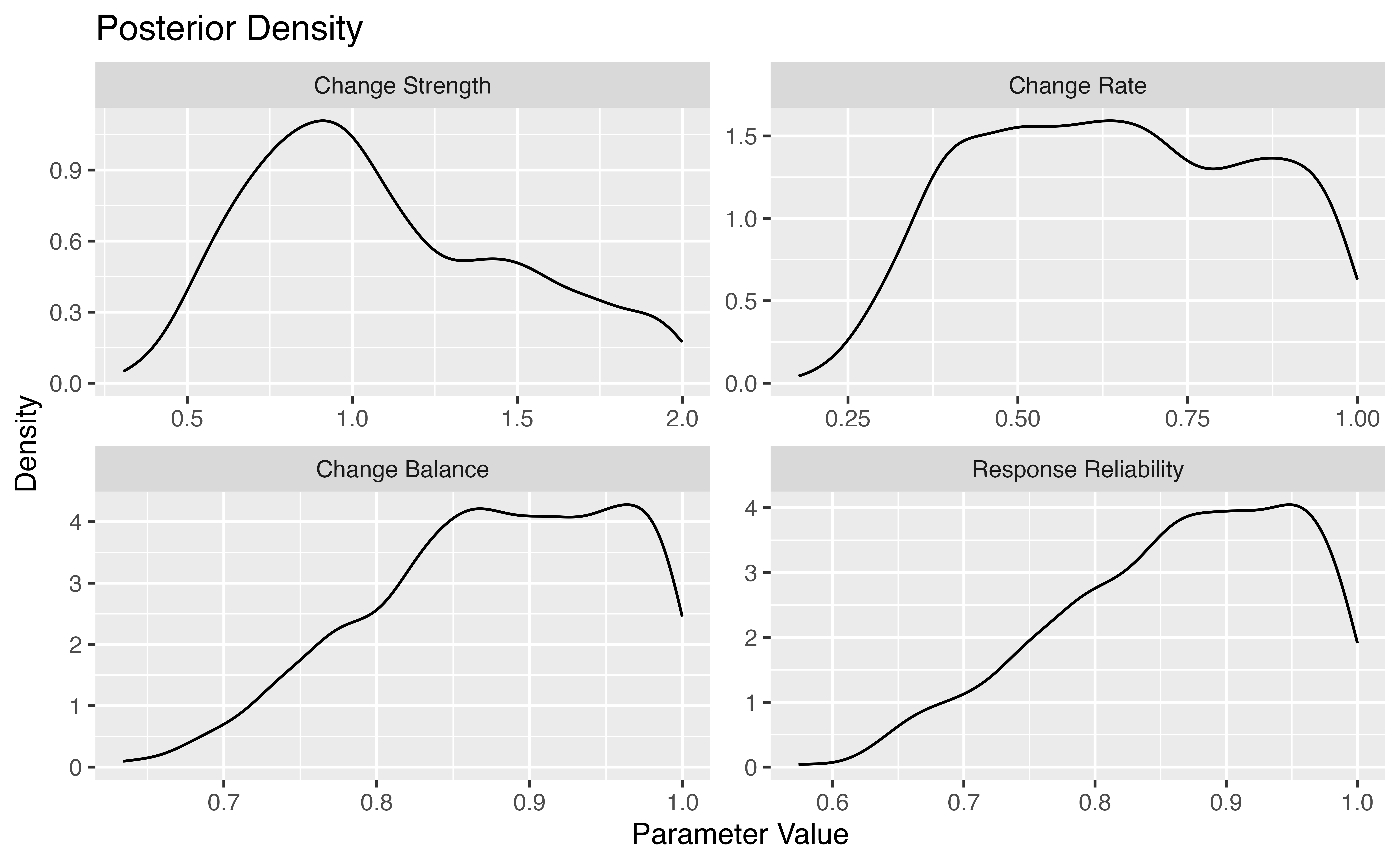
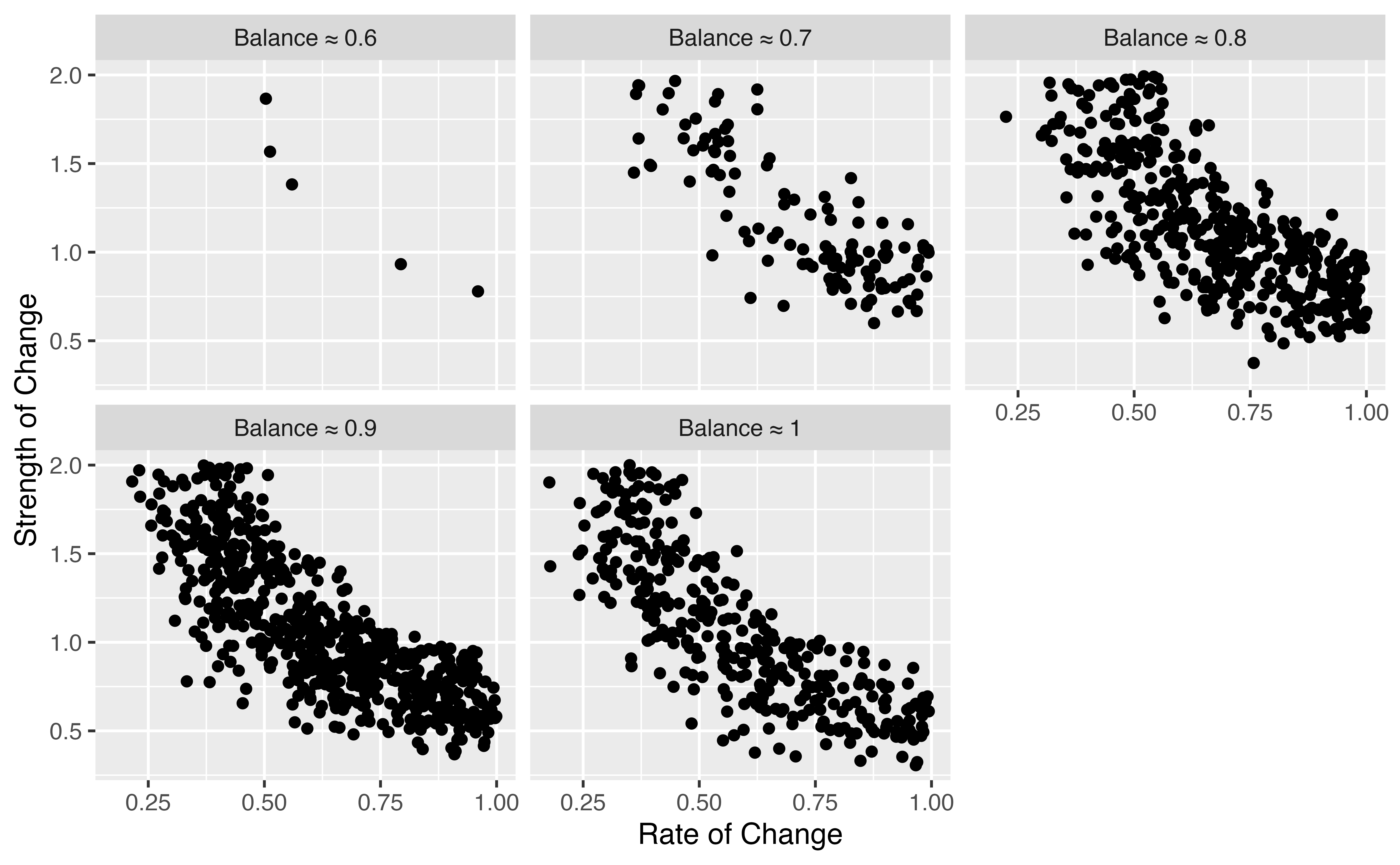
Take the samples that resulted in the smallest distance as plausible DGPs for our observed data. Smaller distances represent a closer resemblance of the simulated to the observed data, indicating that the proposed DGP could have generated our real-world data.

Let’s apply this to our simulated dataset.

grid <- gridSearch(
  data = d,
  yname = 'y', ## observed binary outcome
  tname = 't', ## time variable
  pname = 'p', ## panel identifier
  n_samples = 1e5 ## the number of draws from the priors
)
#> [1] "1%"
#> [1] "2%"
#> [1] "3%"
#> [1] "4%"
#> [1] "5%"
#> [1] "6%"
#> [1] "7%"
#> [1] "8%"
#> [1] "9%"
#> [1] "10%"
#> [1] "11%"
#> [1] "12%"
#> [1] "13%"
#> [1] "14%"
#> [1] "15%"
#> [1] "16%"
#> [1] "17%"
#> [1] "18%"
#> [1] "19%"
#> [1] "20%"
#> [1] "21%"
#> [1] "22%"
#> [1] "23%"
#> [1] "24%"
#> [1] "25%"
#> [1] "26%"
#> [1] "27%"
#> [1] "28%"
#> [1] "29%"
#> [1] "30%"
#> [1] "31%"
#> [1] "32%"
#> [1] "33%"
#> [1] "34%"
#> [1] "35%"
#> [1] "36%"
#> [1] "37%"
#> [1] "38%"
#> [1] "39%"
#> [1] "40%"
#> [1] "41%"
#> [1] "42%"
#> [1] "43%"
#> [1] "44%"
#> [1] "45%"
#> [1] "46%"
#> [1] "47%"
#> [1] "48%"
#> [1] "49%"
#> [1] "50%"
#> [1] "51%"
#> [1] "52%"
#> [1] "53%"
#> [1] "54%"
#> [1] "55%"
#> [1] "56%"
#> [1] "57%"
#> [1] "58%"
#> [1] "59%"
#> [1] "60%"
#> [1] "61%"
#> [1] "62%"
#> [1] "63%"
#> [1] "64%"
#> [1] "65%"
#> [1] "66%"
#> [1] "67%"
#> [1] "68%"
#> [1] "69%"
#> [1] "70%"
#> [1] "71%"
#> [1] "72%"
#> [1] "73%"
#> [1] "74%"
#> [1] "75%"
#> [1] "76%"
#> [1] "77%"
#> [1] "78%"
#> [1] "79%"
#> [1] "80%"
#> [1] "81%"
#> [1] "82%"
#> [1] "83%"
#> [1] "84%"
#> [1] "85%"
#> [1] "86%"
#> [1] "87%"
#> [1] "88%"
#> [1] "89%"
#> [1] "90%"
#> [1] "91%"
#> [1] "92%"
#> [1] "93%"
#> [1] "94%"
#> [1] "95%"
#> [1] "96%"
#> [1] "97%"
#> [1] "98%"
#> [1] "99%"
#> [1] "100%"

head(grid)
#>    ic_sample pc_sample bal_sample rel_sample     error
#>        <num>     <num>      <num>      <num>     <num>
#> 1: 1.5255671 0.7924700 0.58834925  0.7912586 0.1090000
#> 2: 1.2008167 0.3243189 0.70781997  0.9426350 0.0980000
#> 3: 0.1467324 0.5085090 0.09290602  0.4536723 0.1461822
#> 4: 0.4329042 0.1802234 0.31801234  0.1787105 0.2120000
#> 5: 0.7518931 0.5255735 0.54647617  0.1034809 0.1810000
#> 6: 0.4063079 0.3642176 0.06537869  0.7201241 0.1260000

The gridSearch function gives us a data table with five columns:

ic_sample shows the value of the strength parameter informing our DGP,
pc_sample shows the value of the rate parameter informing our DGP,
balance shows the extent to which our sample makes positive changes; put differently, it shows the direction of change in the sample,
rel_sample provides a value of the reliability score retrieved from the search.
error provides the KS distance between observed and simulated trajectories.

Evaluating the Potential DGPs

We can visually inspect the best parameter distributions using gridPlot:

gridPlot(grid, plot = "posterior", cutoff = 0.05)

Alternatively, we can look at the conditional accepted samples:

gridPlot(grid, plot = "conditional", cutoff = 0.05)

Warnings and Notes

We would like to flag a few issues that you need to be aware of:

Currently, gridsearch only accommodates binary outcomes. We are hoping to generalize these procedures to cases where we have more than 2 response categories.
gridSearch requires a balanced panel dataset, with no missing values.

For more details about the protocol, please see the article, The Promises and Pitfalls of Using Panel Data to Understand Individual Belief Change, stored in SocArXiv.