Using the opin Package • opin

Motivation

When public opinion changes over time, there may be three mechanisms driving it:

the mix of cohorts among the population may be changing,
the groups themselves may be changing their opinions, or
both may be happening simultaneously in ways that intensify a specific trend.

opin decomposes aggregate change exactly into these three components, which is useful for understanding the mechanisms behind trends in public opinion.

Illustration

Data Preparation

I use the General Social Survey variable racmar (approval of interracial marriage) to illustrate this approach. The gssr package provides the data.

First, let’s prepare the data for analysis:

library(opin)
library(tidyverse)

## install gssr if not available
if (!requireNamespace("gssr", quietly = TRUE)) {
  install.packages("gssr", repos = c("https://kjhealy.r-universe.dev", "https://cloud.r-project.org"))
}
library(gssr)

## load GSS data
data("gss_all", package = "gssr")

## wrangle
d <- gss_all |>
  select(period = year, cohort, racmar, wt = wtssps) |>
  drop_na() |>
  mutate(
    ## 1 = favor law against racial intermarriage
    racmar = if_else(racmar == 2, 0L, 1L),
    ## choosing 5-year bands for period and cohort values
    period = floor(period / 5) * 5,
    cohort = floor(cohort / 5) * 5
  )

Next, I compute the cohort-level weighted means and population shares. This is the raw data I need for the algebraic decomposition step in the next section.

s <- d |>
  summarise(
    y = weighted.mean(racmar, wt),
    n = n(),
    .by = c(period, cohort)
  ) |>
  mutate(share = n / sum(n), .by = period) |>
  arrange(period, cohort)

## illustrate how the data looks
print(s)
#> # A tibble: 110 × 5
#>    period cohort     y     n   share
#>     <dbl>  <dbl> <dbl> <int>   <dbl>
#>  1   1970   1880 1         5 0.00129
#>  2   1970   1885 0.613    22 0.00569
#>  3   1970   1890 0.757    58 0.0150 
#>  4   1970   1895 0.667   133 0.0344 
#>  5   1970   1900 0.689   184 0.0476 
#>  6   1970   1905 0.482   248 0.0641 
#>  7   1970   1910 0.481   264 0.0683 
#>  8   1970   1915 0.426   308 0.0796 
#>  9   1970   1920 0.440   356 0.0921 
#> 10   1970   1925 0.363   322 0.0833 
#> # ℹ 100 more rows

Decomposition

We can now decompose aggregate change into three components.


## apply
res <- decomp(
  data  = s,
  tname = "period",
  gname = "cohort",
  yname = "y",
  sname = "share"
)

## print
res |> glimpse()
#> Rows: 6
#> Columns: 8
#> $ prev_period <dbl> 1970, 1975, 1980, 1985, 1990, 1995
#> $ curr_period <dbl> 1975, 1980, 1985, 1990, 1995, 2000
#> $ prev_ybar   <dbl> 0.3671661, 0.3221970, 0.2748205, 0.2333722, 0.1643334, 0.1…
#> $ curr_ybar   <dbl> 0.3221970, 0.2748205, 0.2333722, 0.1643334, 0.1163826, 0.1…
#> $ delta_ybar  <dbl> -0.044969010, -0.047376568, -0.041448252, -0.069038812, -0…
#> $ C           <dbl> -0.018299133, -0.045293658, -0.025283959, -0.024954150, -0…
#> $ W           <dbl> -0.024447160, -0.004822172, -0.019482381, -0.042550162, -0…
#> $ R           <dbl> -0.0022227176, 0.0027392624, 0.0033180876, -0.0015344991, …

Each row decomposes the change between consecutive 5-year periods into:

C: composition effect (cohort entry, cohort exit, and cohort share changes),
W: within-cohort attitude change (average change for a cohort compared to previous year),
R: interaction of C and W.

Plotting

opin provides a lightweight function to represent the trends over time:

decompPlot(res)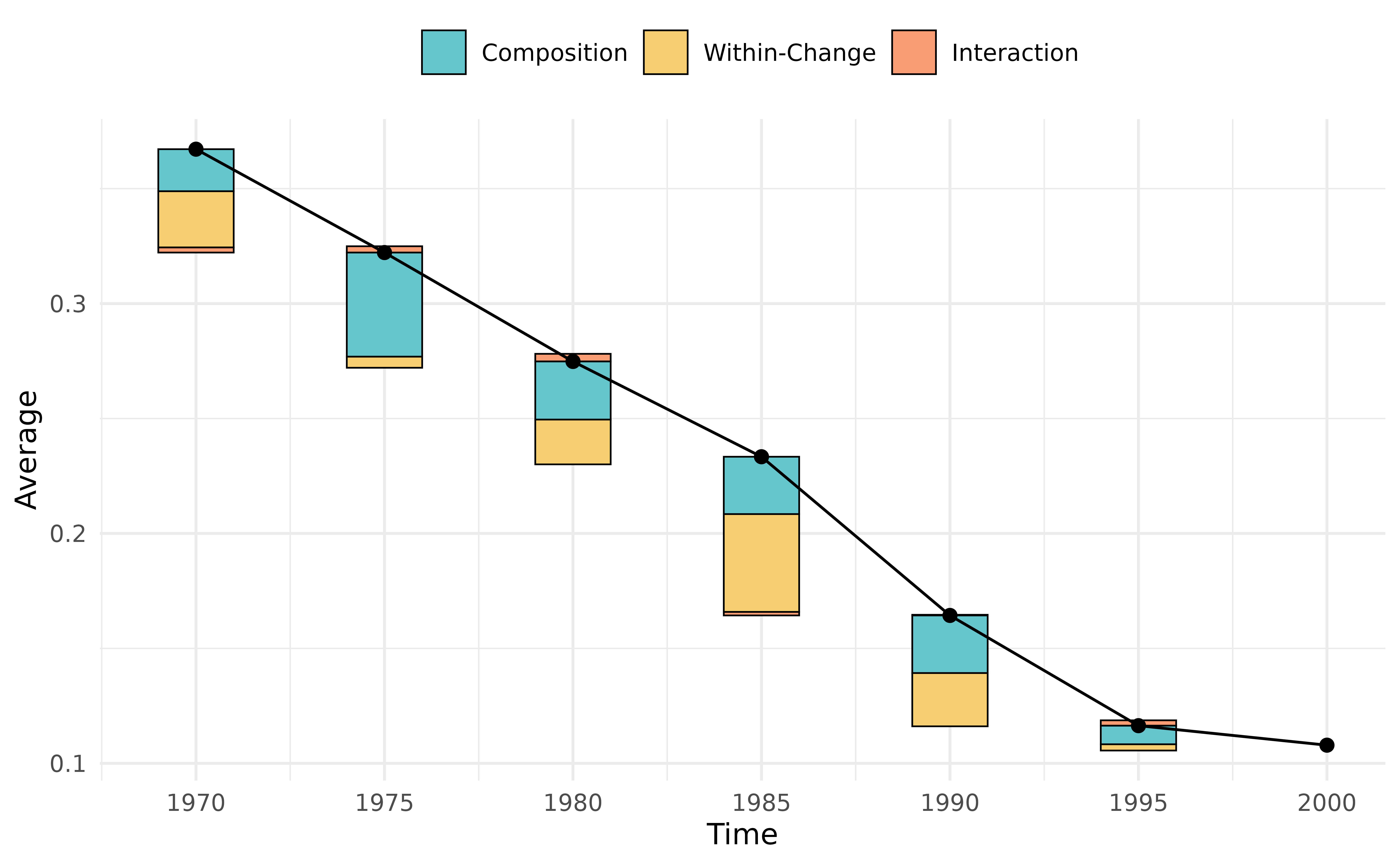

The bars show how much of each period’s change comes from composition (cohort replacement), within-group attitude change, and their interaction. The line traces the aggregate approval rate.

Warnings and Notes

The decomposition is exact, but its interpretation depends on several assumptions:

that within-group entry and exit processes are independent of individual outcomes,
that group boundaries are stable and exogenous, and
that group-level means and shares are measured without error.

These assumptions are unlikely to hold perfectly in most applications, so the exercise should be interpreted as a descriptive look into the data.